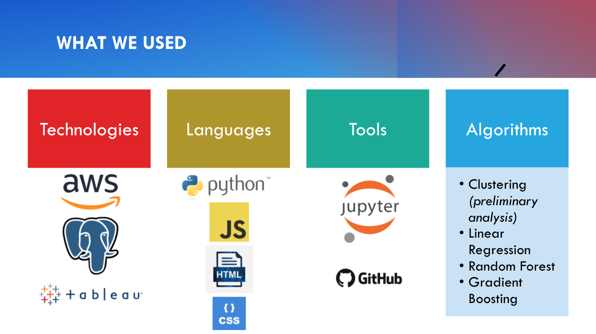
Technologies & Tools Used
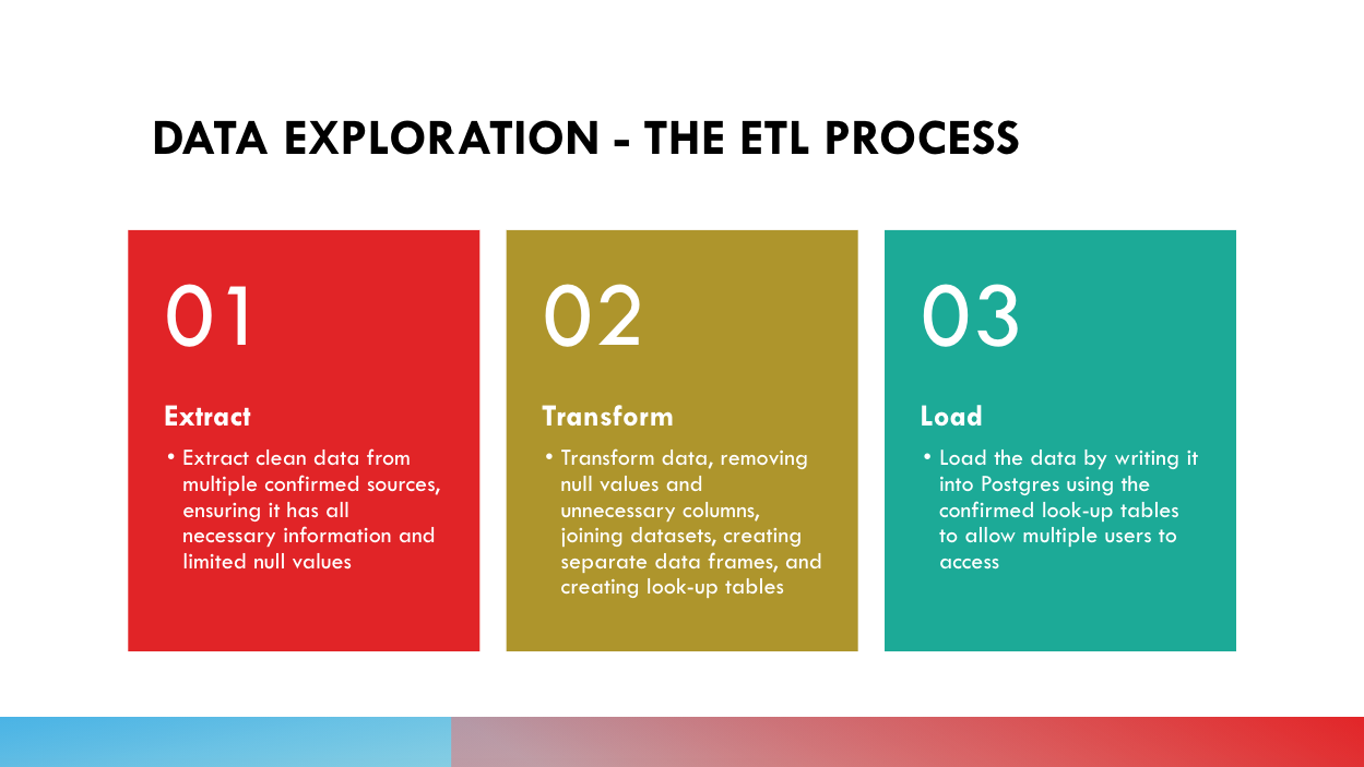
Data Exploration Phase
Data Analysis Phase
Detailed descriptions of our data analysis can be found in our presentation.
Here are the housing price trends of New York (top) and Los Angeles (bottom), after we cleaned null values from our data. We found that the housing prices in Los Angeles to rise in a more linear and predictable fashion compared to New York, which was more sporadic.
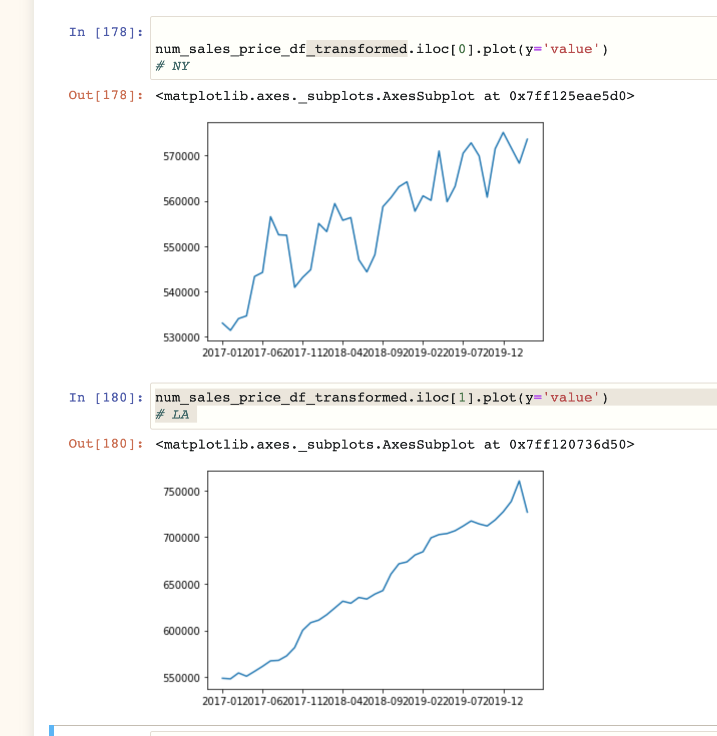
- Looking at two cities, New York and Los Angeles, we found that housing prices have increased over the years, but not steadily for all cities.
- New York’s (top graph) housing market has large increases and decreases in shorter periods of time.
- Los Angeles’s (bottom graph) housing market shows small increases each year, but less decreases.
- When comparing this trend to unemployment rates, Los Angeles has consistently decreased, while New York has fluctuated.
- Preliminary Conclusion: Given the data for New York, it is possible some city housing markets may drop within the next few months, instead of assuming all will continue to rise.
Data Sources
Kaggle: Zillow US House Price Data
Census: US City and Town Population Totals: 2010-2019
Bureau of Labor Statistics: Unemployment Rates by City
Database
-
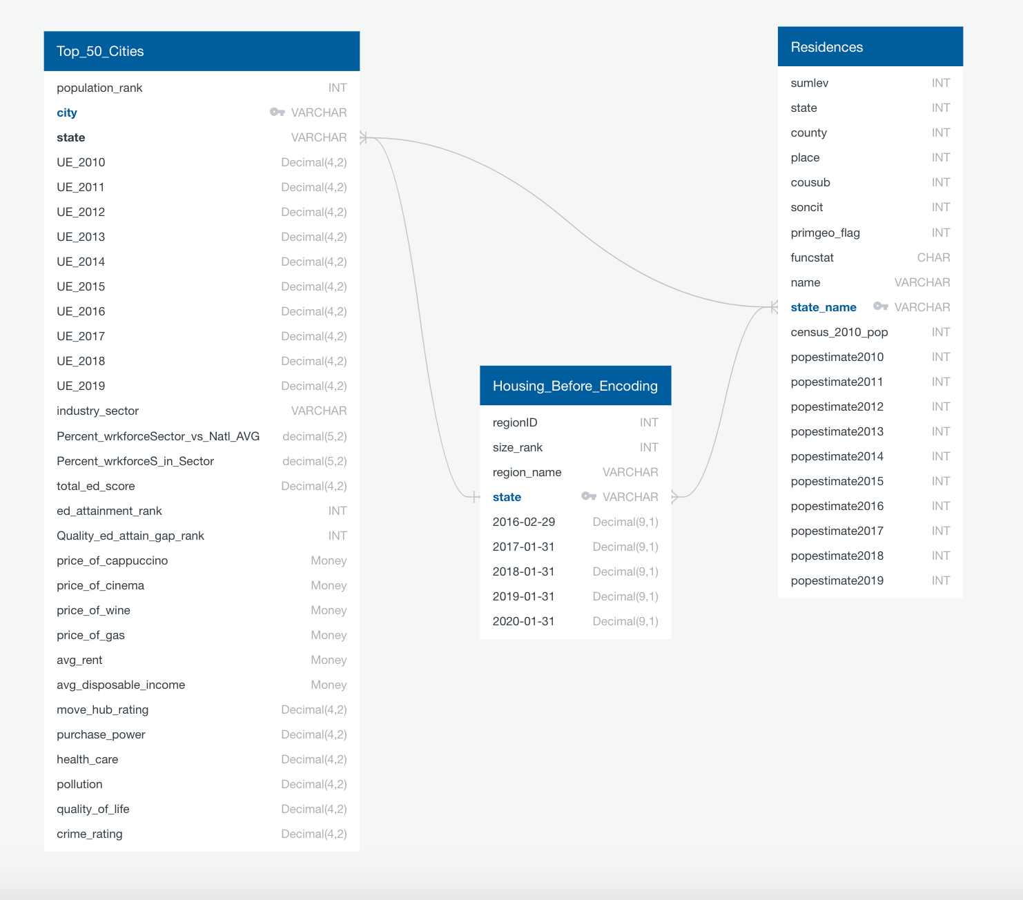
For our database, we will be using PostgreSQL by use of pgAdmin and we are also hosting our raw data in an AWS S3 bucket. This enables anyone with the access codes to work the project data. The image below represents the tables of data that are uploaded onto the database in Postgres. The entity relational diagram allowed for easier joining of tables with SQL and was a helpful reference while importing data into the database. There are three main tables with data that were used to build and perform the machine learning model.
-
The most common and obvious connect between all of our datasets is the State column.
Machine Learning
Preliminary Data Processing
-
The first steps were to check the kind of data types were inside of the CSV file housing our data for each city. We found that our dataset had city name, state, county and average sales price for all home types inside of that city with time steps of months from 2006 to 2020.
-
The next was to check for duplicates and null values in the dataframe we created. We chose to keep the first of each of the duplicates and drop all rows (cities) that had more than 10% null values. This left a little over 17,000 cities with data from the year 2016-2020.
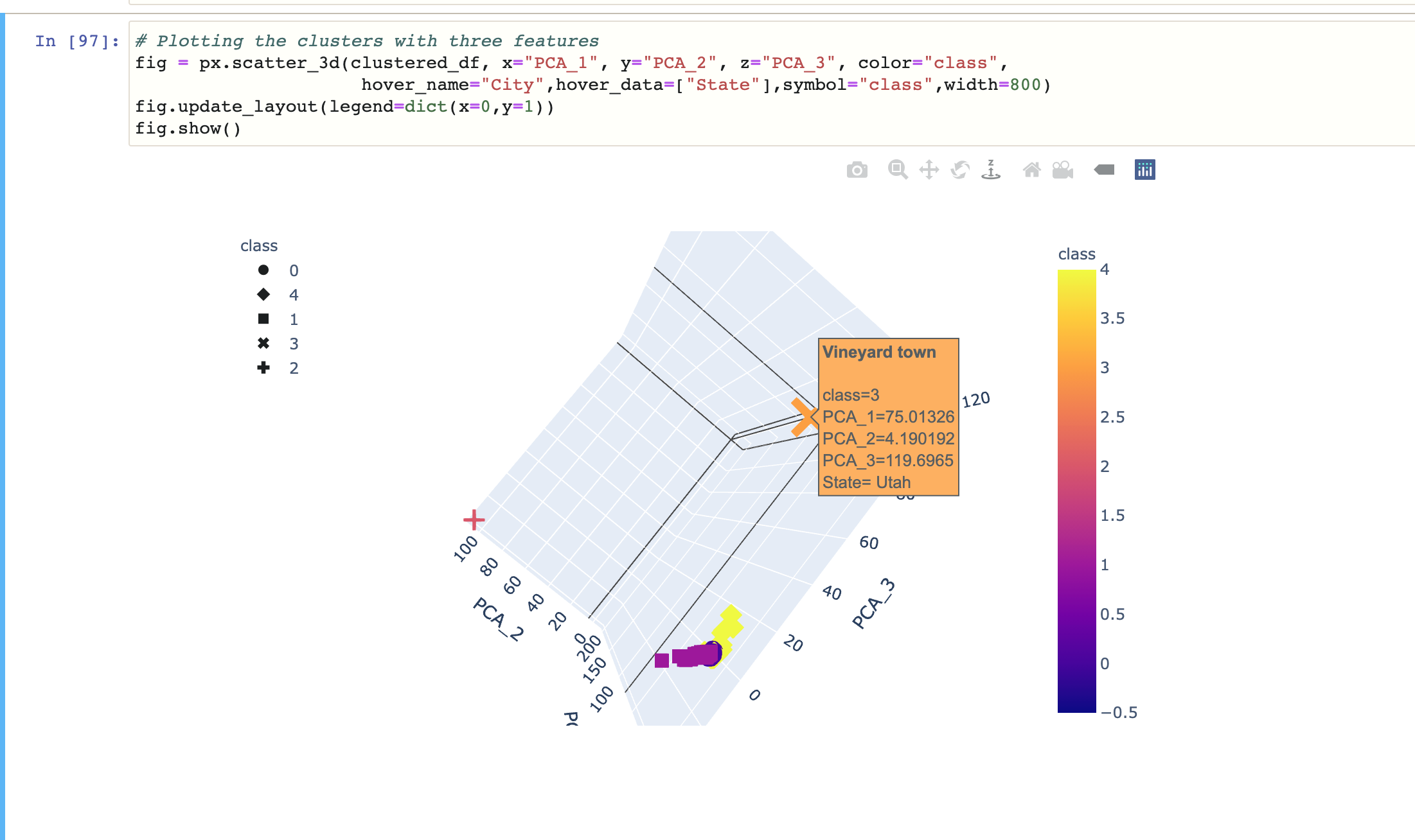
After our preliminary processing, were able to perform an initial unsupervised clustering. We attained the following 3D Pricincipal Cluster Analysis Plot:
-
For the null values we decided to use a KNN (K-Nearest-Neighbors) imputer to fill in the values, as a simple imputer would have used the mean or median housing price. For housing data with large variances between large cities like New York and small towns, we believed that nearest-neighbor medians would not skew the data as much as the median of the whole column.
-
With the 4 years of monthly time-step data for the remaining 17,000 cities, the categorical features of the state that the cities were in was ordinal-encoded, then one-hot-encoded, and finally added into the data frame to be used as a feature with the rest of the time series data. This brought the total number of columns from 177 to 224.
For our final linear regression model, we used an 80/20 testing/training split to achieve our results. The testing/training splits we tried in other methods are shown in the table below.
Explanation of Model Choice (Including Limitations & Benefits)Here are the models we tried, along with results we got:
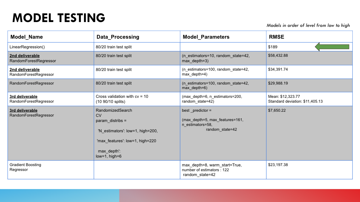
- The Linear Regression model outperformed the closest model by 40x RMSE. Since it was the most simple solution, we tried a few other models as well to see if we could outperform it.
- The second closest was random forest regression that was placed through a stochastic cross validation with a RMSE of $7650.22.
- This model is over 3x more accurate than the other random forest models attempted
- This includes the Gradient BoostingRegressor which is built to optimize validation error, while also stopping training trees before overfitting occurs.